
Searching From Both Ends
In short: running two searches at once — one forward from the start, one
backward from the goal — and stopping when they meet cuts the explored region
from about b^d junctions to about 2·b^(d/2), a square root, not a halving.
With equal edge weights the first meeting point is already the answer. With
different weights, run two Dijkstras and record every crossing between the
two settled regions, stopping only when the two heaps' cheapest remaining
entries add up to at least the best crossing found — the first touch is not
always the cheapest route.
The slowest queries Meridian answers are the cross-city ones: a pickup on the east ring road, a drop-off on the far west. A search from the pickup spreads out in rings, and by the time a ring reaches the drop-off it has swept up most of the city.
Here's a better idea. Start a second search from the drop-off at the same time, and stop when the two meet in the middle. Two small circles instead of one big one. On a network where each junction branches out, that is not a small saving, and this lesson shows how big it is. It also shows the one detail that makes the weighted version subtle: the moment the searches first touch is not always the moment you have the answer.
Why two halves beat one whole
Suppose every junction leads to about b new junctions, and the route is d roads long. A search from one end explores roughly b to the power d junctions before it arrives. Two searches that each go halfway explore about 2 × b to the power d/2:
That's a square root, not a halving:
b, d = 3, 8
print(b ** d, 2 * b ** (d // 2))Here's the difference as the route gets longer, when each junction leads to 3 new ones:
| route length d | one search (3^d) | two searches (2 × 3^(d/2)) | ratio |
|---|---|---|---|
| 4 | 81 | 18 | 4.5 |
| 8 | 6,561 | 162 | 40.5 |
| 14 | 4,782,969 | 4,374 | 1,093.5 |
| 20 | 3,486,784,401 | 118,098 | 29,524.5 |
The ratio is 3 to the d/2, over 2, so every two extra roads triple it, and at 14 roads it passes a thousand. City routes of 30 or 40 roads make the one-sided search millions of times more expensive, at least until the network's edges stop the frontier growing.
Two BFS searches, unweighted
With every road counting as 1, run a BFS from each end. Each round, grow the side with the smaller frontier by one whole ring, since that's the cheaper side to grow. The moment a ring reaches a junction the other side has seen, the route length is the sum of the two hop counts.
In code, keep one hops dict and one frontier list per side, indexed 0 and 1, so the
same loop body serves both directions:
With every road costing 1, the first touch is the answer: both searches grow a whole ring at a time, so no shorter crossing can still be hiding.
Watch it on a stretch of Meridian: a ring road where every junction also has one cross-town link. The forward search's junctions are badged F, the backward search's B:
Your bidirectional BFS. Two frontiers each grow halfway, and together touch half the junctions one search needs.
Try changing the goal to "j18", or the cross-town rule from i * 8 + 14 to
i * 3 + 5, and compare the two counts in the last frame. On a plain grid, where
rings grow only linearly, the saving shrinks to about half. It's biggest where the
network branches.
With weights, meeting isn't finishing
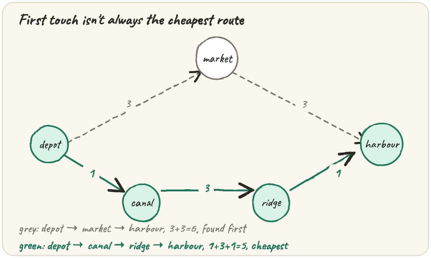
Now let roads have different costs, and run two Dijkstras. Growing the side with the cheaper next pop keeps both searches roughly the same "radius". The tempting rule is to stop as soon as some junction is settled by both searches. That rule is wrong, and here is the smallest network that shows it:
The searches first touch at the market, but the cheapest route crosses between them along the canal–ridge road. Only a threshold rule knows when to stop.
Forward Dijkstra from the depot, backward Dijkstra from the harbour. Badges show each side's cost. 5 nodes, 5 edges, undirected. depot: F0, harbour: B0.
Two things make it right:
- Record every crossing. Whenever a road joins a junction one side has settled
to a junction the other side has reached, that's a complete route. Keep the
cheapest as
best. - Stop on a threshold. Any route you haven't seen yet must leave the forward
region at a cost of at least the forward heap's smallest entry, and enter the
backward region at a cost of at least the backward heap's smallest. So once
top_forward + top_backward >= best, nothing unseen can win.
Here is the tempting rule, in code. It stops at the first junction both sides settle:
This prints 6, the route through the market. The cheapest route, depot → canal → ridge → harbour, costs 5. Record every crossing and use the threshold rule to stop.
Many starts at once: multi-source search
The opposite trick is just as useful. To find, for every junction, the distance to its nearest depot, don't run one search per depot. Put every depot in the queue at distance 0 and run one BFS. The frontiers grow together, and each junction is claimed by whichever arrives first:
It's the same as adding a hidden junction joined to every depot by a free road and searching from that. The drill exercise builds it.
Two weights only: 0-1 BFS
Some Meridian queries count surcharges: roads on the contracted network are free, others cost 1. Dijkstra works, but with only two weights a deque replaces the heap. A free road leads to a junction at the same cost, so it goes to the front; a surcharged road leads one higher, so it goes to the back:
from collections import deque
roads = {"depot": [("mill", 1), ("canal", 0)], "canal": [("quay", 0)],
         "quay": [("mill", 0)], "mill": []}
best = {"depot": 0}
queue = deque(["depot"])
while queue:
    node = queue.popleft()
    for nxt, w in roads[node]:
        if best[node] + w < best.get(nxt, float("inf")):
            best[nxt] = best[node] + w
            queue.appendleft(nxt) if w == 0 else queue.append(nxt)
print(best["mill"])That runs in O(V + E), no log factor. The build exercise asks you to write it.
Every variant here keeps one hops/dist entry and one frontier slot per
visited junction, on each side: O(V) space whether it's one BFS, two, or a
deque. The saving bidirectional search buys is entirely in time — fewer
junctions ever get visited in the first place.
Interview-style: where should two couriers meet?
Two couriers start at different junctions and must hand over a parcel. They drive at the same time; the handover happens when the later one arrives. Which junction gives the earliest handover?
It's tempting to take the shortest route between them and pick its middle. But the best junction may be off that route, somewhere both can reach quickly. Search from both ends: one Dijkstra from each courier gives every junction's two arrival times, and the answer minimises the later of the two. The boss exercise builds it.
What it costs
| Work | Note | |
|---|---|---|
| One-sided BFS / Dijkstra | about b^d junctions | explores behind the start as much as ahead |
| Bidirectional search | about 2 b^(d/2) | needs the goal known, and the reverse graph for one-way roads |
| Multi-source BFS | O(V + E), any number of sources | distances to the nearest source |
| 0-1 BFS | O(V + E) | weights 0 and 1 only |
❓ Cross-question — "Can you combine this with A*?" Yes, but carefully: each side needs its own heuristic, and the stopping rule has to account for both. Real route planners do combine them, usually with landmark heuristics like the ones in the previous lesson's capstone.
Quick practice
b, d = 2, 10
print(b ** d, 2 * b ** (d // 2))depot and harbour are connected (depot → mill → plaza → harbour, 3 roads), but this returns -1. Fix which side the touch check reads.
🎯 Your turn
Write meet_in_middle(roads, start, goal). roads are two-way [a, b, minutes].
Run Dijkstra from both ends, always popping from the side with the cheaper next
entry, record every crossing, and stop when the two heap tops add up to at least
the best crossing. Return the cheapest cost, 0 if start == goal, or -1:
meet_in_middle([["depot", "market", 3], ["market", "harbour", 3], ["depot", "canal", 1], ["canal", "ridge", 3], ["ridge", "harbour", 1]], "depot", "harbour")→5
Hint: keep dist, heaps and done as two-element lists indexed by side, so
the forward and backward code is the same code.
Then press ▶ Run, tap the Live App try chips to call it with different inputs, and hit ✓ Check. Green = this piece of Meridian's router is built. ✅