
B-Trees and the Disk
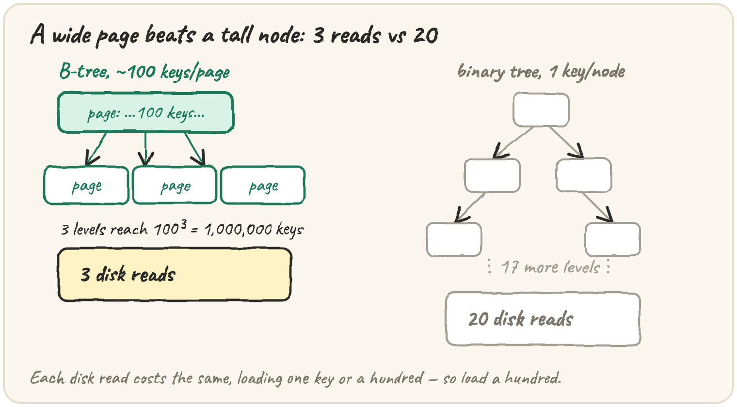
In short: on disk the unit of cost is a page read, not a comparison, so a B-tree packs hundreds of sorted keys into each node instead of one, keeping a million keys in about 3 levels instead of a binary tree's 20. Searching binary-searches inside each loaded page, then follows the child between the two keys that bracket the target. Inserting always goes into a leaf; when a page overflows it splits around its median key, which moves up into the parent — height only ever grows at the top, so every leaf stays at the same depth with no rebalancing pass.
Everything in this section so far has assumed the log fits in memory. Quarry's does, for a while. Then someone asks for a year of per-second events, which is 31 million rows with several fields each, and the index has to live on disk.
Disk changes the cost model, and the change is big enough to change which structure is best:
| operation | rough time |
|---|---|
| read a value already in memory | ~0.0001 ms |
| read a page from an SSD | ~0.1 ms |
| read a page from a spinning disk | ~10 ms |
A disk never hands you one value. It hands you a page, usually 4 to 16 KB, whether you wanted one number from it or all of it. So on disk the thing to count is page reads, not comparisons. Comparing keys inside a page you've already loaded is nearly free by comparison.
Why a binary tree is the wrong shape
A balanced binary search tree over a million keys is about 20 levels deep. On disk each node is a separate page, so every lookup is about 20 page reads, and a range scan hops between pages scattered all over the disk. The binary tree is short enough in memory, but it wastes almost every page it reads: it loads 16 KB to look at one key and two pointers.
The fix is to use the whole page. Put hundreds of sorted keys in each node,
with a child pointer between every pair of neighbouring keys. A node with k
keys has k + 1 children, and child i holds every key strictly between key
i − 1 and key i. That's a B-tree. With about 256 children per page, a
million keys fit in 3 levels, and the top level or two are read so often that
they stay cached in memory. A lookup costs one or two real disk reads.
Put numbers on it. Change the fanouts, or the number of keys:
Searching
At each page, find where the key would go among the page's sorted keys, with a binary search that runs in memory. Either it's there, or you know exactly which child to read next. Here's a small B-tree with at most 3 keys per page. Each node below is one page on disk:
Each box is one page. A search reads one page per level, so the height of the tree is the number of disk reads.
Look for 57. Read the root page. 57 is bigger than 30 and smaller than 60, so it can only be in the middle child. 14 nodes, 13 edges, directed. At 30 60. Settled: 30 60.
reads = 1
n, fanout = 1_000_000, 100
levels, reach = 0, 1
while reach < n:
    reach *= fanout
    levels += 1
print(levels)Inside a page, bisect picks the child. bisect_right(keys, x) counts the keys
at most x, which is exactly the index of the child to follow:
from bisect import bisect_left, bisect_right
keys = [20, 40, 60]
print(bisect_right(keys, 45), bisect_left(keys, 40))That equality check is easy to forget, because in a binary search tree you'd check the node before choosing a side. In a B-tree the keys in internal pages are real keys too:
30 is stored in the root page, so this should print True. It prints False, because the search goes straight past the root to a leaf.
Now write the search yourself. The code turns the nested pages into a graph
for drawing, then walks them. Change key and run it:
Your page search. Every highlighted page is one disk read.
Inserting: split, and grow at the top
A new key always goes into a leaf, in sorted position. If the leaf now holds more keys than a page allows, split it: the median key moves up into the parent, the keys to its left become one page, and the keys to its right another. If that makes the parent overflow, it splits too, and so on up.
A full page takes one more key, then splits around its median. The median becomes a separator in the parent page.
A leaf page holding 25, 30 and 35, with room for at most 3 keys. Insert 33. 3 cells. At index 0.
When the root splits, a new root is made above it holding just the median, and the tree gains a level. That's the only way a B-tree gets taller. Because height is only ever added at the top, every leaf stays at the same depth. The tree is balanced by construction, with no rotations and no rebalancing pass. Step through the split arithmetic:
❓ Cross-question — "Why not a sorted array on disk and binary search?" Lookups would be fine: about 20 reads for a million keys, fewer with caching. But inserting into the middle of a sorted array on disk shifts everything after it, O(n) page writes. A B-tree insert writes one leaf, plus a few pages when it splits. It keeps the sorted order, so it keeps range scans, and it makes inserting cheap.
How wide does a page need to be? A binary tree over a million keys is about 20 levels deep. A B-tree with fanout f is about log base f of a million:
| fanout f | levels for 1,000,000 keys |
|---|---|
| 2 | 19.9 |
| 10 | 6 |
| 50 | 3.5 |
| 100 | 3 |
| 400 | 2.3 |
A hundred children per page is the smallest fanout that fits a million keys in three levels, since 100³ = 1,000,000. Real pages of 16 KB with 8-byte keys and pointers hold several hundred, so databases typically sit at 3 or 4 levels even for billions of rows.
Idioms & real-world patterns
Range scans, and why most databases use a B+ tree
A range query, "every key from 40 to 57", visits only the children whose key ranges overlap the query and skips the rest. That's the same total-cover, partial, disjoint reasoning as the segment tree, applied to a wider node. Most databases use a B+ tree variant: every record lives in the leaves, internal pages hold only separators, and each leaf points to the next leaf. A range scan then finds its first leaf with a normal search and reads leaves in order until it passes the end: one search, then one read per page of results.
Why the root is (nearly) free
The root page is read on every single lookup, so it's always in the cache, and the next level usually is too. On a three-level tree most lookups do a single real disk read, for the leaf.
Quick practice
n, fanout = 1_000_000, 1000
levels, reach = 0, 1
while reach < n:
    reach *= fanout
    levels += 1
print(levels)Splitting [10, 20, 30, 40] should push up 30 and leave 40 as the only key on the right, but this prints (30, [10, 20], [30, 40]) — 30 is still sitting in both the parent and a leaf.
🎯 Your turn
Build Quarry's page index: page_search(tree, key). A page is
{"keys": [...], "children": [...]} with sorted keys. A leaf has
"children": [], and an internal page with k keys has k + 1 children. Return
{"found": True or False, "reads": pages_read}, where every page you look at
counts as one read, and stop as soon as the key is found.
- For the lesson's tree,
page_search(tree, 57)→{"found": True, "reads": 3}andpage_search(tree, 30)→{"found": True, "reads": 1}
Then press ▶ Run, tap the Live App try chips to call it with different inputs, and hit ✓ Check. Green means this piece of Quarry is built. ✅