
B-Trees, the Disk, and the 2-3 Tree
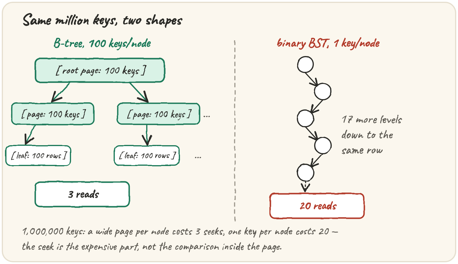
In short: a binary tree wastes disk reads. Every level is one more seek — a real, millisecond-scale trip to storage — so a binary tree over a million keys costs 20 seeks to find one row. A B-tree widens each node to hold many keys and many children (a "page" sized to match one disk read), so the same million keys cost 3 or 4 seeks, not 20. The 2-3 tree is the smallest useful B-tree — every node holds 1 or 2 keys and has 2 or 3 children — and it's a good place to see why branching factor matters before looking at a real, wide disk index.
Why database indexes use B-trees, not BSTs
Every real database (Postgres, MySQL, SQLite) indexes rows with a B-tree, not a binary search tree. The reason is physical: reading one disk page costs about the same whether it holds 2 keys or 200, because the expensive part is the seek, not reading the extra bytes once you're there. A wide node wastes almost nothing and saves a whole level.
A filesystem's directory index
A filesystem (NTFS, most of ext4's modern layout, APFS) stores a directory's entries — thousands of files, sorted by name — in a B-tree on disk too, for the same reason a database does: listing or looking up a file by name should cost a handful of reads, not one per comparison. The mistake people actually make reasoning about this: assuming a wider node is "more work" because it holds more data, instead of noticing that the read itself — not the comparisons inside it — is the expensive step.
def seeks_for(n, max_keys):
    import math
    branching = max_keys + 1
    depth, capacity = 0, 1
    while capacity < n + 1:
        capacity *= branching
        depth += 1
    return depth

# A directory with 50,000 files, compared at two page sizes
print(seeks_for(50_000, 4), seeks_for(50_000, 200))The 2-3 tree: the smallest useful B-tree
In Knuth's standard terminology, a B-tree's order counts the maximum
number of children a node can have, not keys. A 2-3 tree — every node
holds 1 or 2 keys and has 2 or 3 children — is therefore a B-tree of
order 3, not "order 2". To dodge that off-by-one trap in every example,
this lesson's code parameterises by max keys per node instead (a 2-3
tree is max_keys = 2; a page holding up to 100 keys is max_keys = 100,
order 101 in Knuth's sense). A 1-key node looks exactly like a binary BST
node. A 2-key node is the new shape — [a | b] with three
children: everything less than a, everything between a and b, and
everything greater than b. That third child is the whole idea of a
B-tree in miniature: one more key buys one more branch.
Max-keys-per-node doesn't just mean "store more per node" — it's the whole
reason a B-tree stays shallow. Going from max_keys=2 (2-3 trees, order 3)
to max_keys=100 (a real disk page, order 101) doesn't make each node 50x
more expensive to read (it's still one disk seek); it makes the tree 50x
wider at every level, which is where the seek count actually comes from.
import math

def btree_depth(n, max_keys):
    if n <= 0:
        return 0
    branching = max_keys + 1
    depth, capacity = 0, 1
    while capacity < n + 1:
        capacity *= branching
        depth += 1
    return depth

print(btree_depth(1_000_000, 2), btree_depth(1_000_000, 100))Quick practice
def child_for(node_keys, target):
    for i, key in enumerate(node_keys):
        if target < key:
            return i
    return len(node_keys)

print(child_for([5, 15, 25], 30))import math
print(math.ceil(math.log2(1_000_001)) == 20)What it costs
| structure | depth for 10⁶ keys | disk reads per lookup |
|---|---|---|
| balanced binary BST | ~20 | ~20 |
| 2-3 tree (max_keys=2, Knuth order 3) | ~13 | ~13 — better, but each node is still a tiny fraction of a disk page |
| B-tree, 100 keys/node (Knuth order 101) | 3 | 3 — one node fills a whole disk page |
| plain sorted array (binary search) | ~20 comparisons | up to ~20 reads, unless the whole array is cached |
🎯 Your turn
Build tree_depth_comparison(n, order): report the depth of a B-tree of
the given order (max keys per node) over n keys, alongside a binary
BST's worst case (n, fully degenerate) and best case (balanced). Return
{"btree_depth": ..., "bst_worst_depth": ..., "bst_balanced_depth": ...}.
tree_depth_comparison(1000000, 100)→{"btree_depth": 3, "bst_worst_depth": 1000000, "bst_balanced_depth": 20}tree_depth_comparison(7, 2)→{"btree_depth": 2, "bst_worst_depth": 7, "bst_balanced_depth": 3}
Hint: btree_depth grows the tree's capacity by a factor of
order + 1 per level until it reaches n + 1; bst_balanced_depth is
ceil(log2(n + 1)); bst_worst_depth is just n.
Press ▶ Run, then ✓ Check.