
Randomness as an Algorithm
In short: a fixed pivot rule has some input that defeats it, and a chart that arrives already sorted is exactly that input for "always pick the last value". Picking the pivot at random removes the input from the equation: no input is bad any more, only bad luck is, and the chance of real bad luck shrinks to nothing as n grows. The same idea — remove the fixed rule an adversary (or an unlucky dataset) could aim at — also underlies a fair shuffle, reservoir sampling and Python's own hash randomisation.
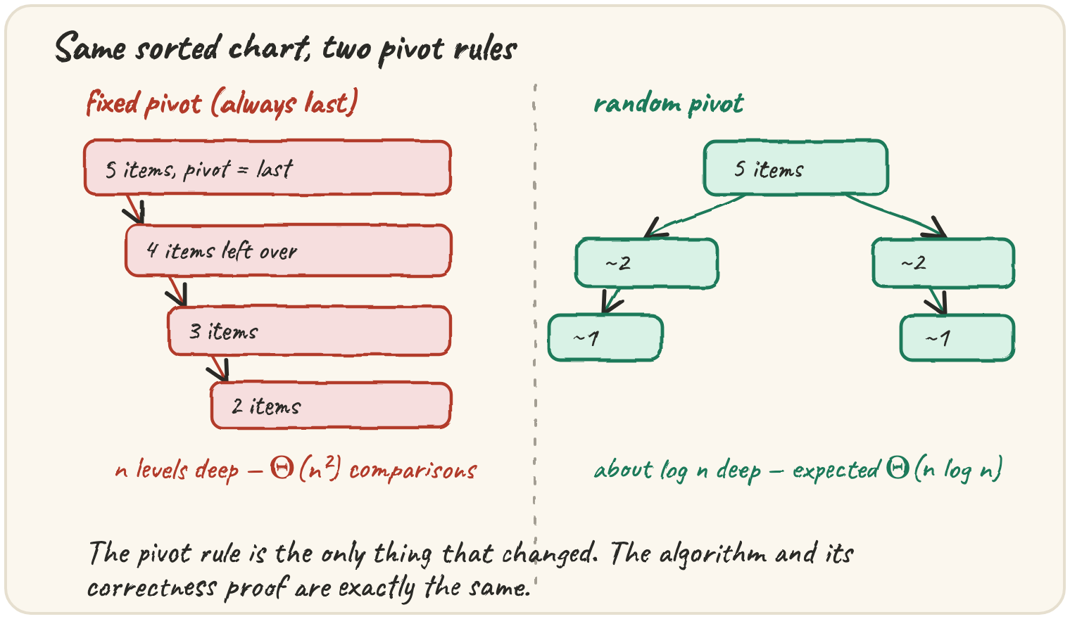
Tunebox's weekly chart arrives already sorted by last week's position, and a lot of it barely moves. In section 3 you saw what that does to a quick sort that always takes the last value as its pivot: every pivot is the largest value left, every partition peels off one item, and the sort does comparisons. On a chart of 64 tracks that is 2,016 comparisons where about 360 should do.
You could pick a cleverer fixed pivot, such as the middle, but any fixed rule has some input that defeats it, and somebody's data will be that input. This lesson takes the rule away from the input: let a random number pick the pivot. Then no input is bad. Only bad luck is, and you can measure exactly how unlikely it is.
One line changes
Here is your section 3 quick sort with its pivot choice pulled out into a function.
It runs on a sorted chart of 10 tracks. The seeded generator makes the "random"
choices the same on every run, so you can compare. Edit choose_pivot: try
return hi, the old rule, and watch the comparison count jump.
Your quick sort with a random pivot on a chart that is already sorted. The pivots land near the middle, so the ranges halve.
The only change from section 3 is two lines: pick an index at random, and swap that value into the pivot slot before partitioning. Everything else, including the correctness argument, is untouched. Whatever the random choices are, the output is sorted:
import random

rng = random.Random(2024)
chart = ["Aria", "Blue", "Cove", "Dawn", "Echo"]
shuffled = list(chart)
for i in range(len(shuffled) - 1, 0, -1):
    j = rng.randint(0, i)
    shuffled[i], shuffled[j] = shuffled[j], shuffled[i]
print(sorted(shuffled) == chart)Measuring the luck
One run proves nothing about a random algorithm. Run it 200 times on the same sorted chart of 64 tracks and look at the spread of comparison counts:
The fixed rule costs 2,016 on this input, every single time. The random rule's worst run out of 200 is still under a third of that, and most runs sit near the middle of the bell. The input no longer matters. What varies is the coin flips, and they are on your side.
Why the expectation is n log n
Name the values 1 to n in sorted order. Two values i < j are compared only if one of them is the first pivot chosen from the range i, i+1, …, j. If any value strictly between them is picked first, it sends i and j to opposite sides and they never meet. Each of the j − i + 1 values in that range is equally likely to be first, so
Step through it for the values 2 and 6 in a chart of 8:
Two values meet only if one of them is the first pivot drawn from the range between them, so close values meet often and distant ones rarely.
Will quick sort ever compare the values 2 and 6? 8 cells.
Adding that over every pair gives the expected number of comparisons. For three values:
from fractions import Fraction

n = 3
expected = sum(Fraction(2, j - i + 1)
               for i in range(1, n + 1)
               for j in range(i + 1, n + 1))
print(expected)Summed for general n, the pairs a distance d apart contribute about each, and is the harmonic number . So the expectation is about . The same number falls out of a recurrence, averaging over the n equally likely pivot positions:
For n = 64 that is 360.7, close to the median of the 200 runs above.
❓ Cross-question — "Can a random pivot still hit the n² case?" Yes, if every pivot happens to be the largest value left. The chance of that is : for 64 tracks, about one in . More usefully, the probability of doing even twice the expected work shrinks exponentially with n.
Las Vegas and Monte Carlo
Random quick sort is a Las Vegas algorithm: the answer is always right, and only the running time is random. The other kind, a Monte Carlo algorithm, has a fixed running time and an answer that is only probably right, or only approximately.
Tunebox's smart shuffle (section 3's capstone) exists because a plain shuffle often plays the same artist twice in a row. How often? Counting all the orders exactly is hard. Sampling them is easy:
The estimate settles as the trials grow, but slowly: the typical error of a sampled fraction shrinks like for t trials. Ten times more precision costs a hundred times more trials.
How many shuffles must the estimate use for its typical error to be about 1%?
| trials t | typical error 1/√t |
|---|---|
| 100 | 10% |
| 500 | 4.5% |
| 1,000 | 3.2% |
| 10,000 | 1% |
| 100,000 | 0.32% |
It takes 10,000. Going from 500 trials to 10,000 is twenty times the work for about four and a half times the precision. That square root is the price of every Monte Carlo estimate.
A fair shuffle is a randomised algorithm too
rng.shuffle is the Fisher–Yates shuffle: walk from the last position down, and
swap each position with a uniformly random position at or before it. Each of the
n! orders comes out with probability exactly . Get the range slightly wrong
and some orders can never happen:
Three tracks have 6 possible orders, and 3,000 fair shuffles should produce all of them. This version only ever produces 2, because no track can stay where it is.
Picking one from a stream
Some choices can't see the whole list first. Tunebox's radio wants one song chosen uniformly from a live stream of plays, without storing the stream. Reservoir sampling keeps a single pick: the k-th item replaces it with probability 1/k. Step through it on five plays:
The k-th item is picked with probability 1/k and then survives every later item m with probability . Multiply those and everything cancels to : each song is equally likely, and the memory is one variable.
Idioms & real-world patterns
Seed it in tests, not in production
random.Random(seed) gives a private generator whose sequence is the same on every
run. Use a seed in tests and demonstrations so failures reproduce. In production
leave it unseeded; a fixed seed turns "random" back into a fixed rule, and a fixed
rule can be attacked.
random.shuffle, random.sample, random.choices
Use the library: shuffle is Fisher–Yates in place, sample(pop, k) draws without
replacement, and choices(pop, weights, k=…) draws with replacement by weight.
Hand-rolled versions are where the off-by-one bias lives.
⚡ Advanced — randomness against attackers
A hash table can be attacked with keys chosen to collide. Python randomises its
string hashing per process (PYTHONHASHSEED) so an attacker can't precompute
colliding keys. It is the random pivot idea again: remove the fixed rule the
adversary would aim at.
Quick practice
from fractions import Fraction

n = 4
expected = sum(Fraction(2, j - i + 1)
               for i in range(1, n + 1)
               for j in range(i + 1, n + 1))
print(expected)With this seed, correct reservoir sampling (one replacement in k) picks "blue". This prints "aria", because randint(0, k) makes the replacement chance 1/(k+1), not 1/k.
🎯 Your turn
Write quicksort_cost(items, seed), the cost lab's pivot lab. Sort a copy of
items with your quick sort and return how many comparisons it made. Use
rng = random.Random(seed), and in every partition of lo..hi (with lo < hi)
pick p = rng.randint(lo, hi), swap items[p] into hi, then partition exactly as
in section 3: one comparison items[j] < pivot per j from lo to hi - 1. Recurse
on the left side first.
quicksort_cost([5, 3, 8, 1, 9, 2], 1)→9quicksort_cost(list(range(64)), 5)→347, a sorted chart nowhere near 2,016
Then press ▶ Run, tap the Live App try chips, and hit ✓ Check.