Capstone — Quarry's Query Planner

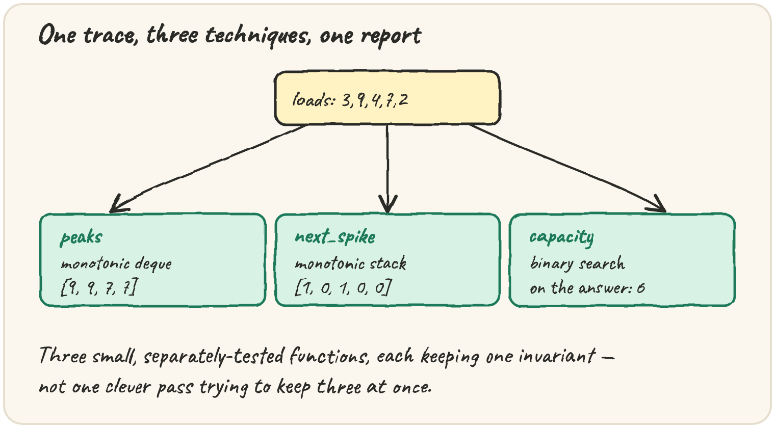
In short: plan_capacity reads one load trace and answers three questions, each with a technique from this section: a monotonic deque for the window peaks, a monotonic stack for the wait until the next heavier tick, and a binary search on the answer — backed by a simulation — for the smallest capacity that keeps the backlog inside its promise. Keep the three as small, separately-tested functions rather than one clever merged pass, prove the search's monotonicity by comparing two runs, and settle the edge cases (an empty trace, a window of zero, a promise of zero) before writing a line.

One load trace feeding three techniques: a monotonic deque for peaks, a monotonic stack for next_spike, and a binary search on the answer for capacity

Every piece of this section answered one question about a trace. The planner answers three at once, and it has to answer them fast enough to run on every refresh of Quarry's operations page. It reads a load trace: loads[t] is how many units of query work arrived at tick t.

What you're building

plan_capacity(loads, k, sla) -> {"peaks": [...], "next_spike": [...], "capacity": c}

plan_capacity([3, 9, 4, 7, 2], 2, 4)
# {"peaks": [9, 9, 7, 7], "next_spike": [1, 0, 1, 0, 0], "capacity": 6}

peaks: the heaviest load in every window of k consecutive ticks, for the dashboard. That's the monotonic deque from lesson 2. With k less than 1 or longer than the trace, it's [].
next_spike: for each tick, how many ticks until a strictly heavier load arrives, or 0 if none does. That's the monotonic stack from lesson 1.
capacity: the smallest whole number of units per tick, at least 1, that a server can process while keeping the backlog at or below sla after every tick. That's a binary search on the answer from lesson 3, with a simulation as its check.

Each part is a technique you've already written. The work in a capstone is getting their edges right, proving the one fact the search relies on, and keeping the whole thing O(n log L), where L is the heaviest load.

The backlog model

A server with capacity c clears up to c units per tick. Whatever it can't clear waits for the next tick, and a quiet tick can't bank unused capacity for later:

python

With c = 5 the backlog reaches 5 at tick 3, which breaks a promise of 4. With c = 6 it never passes 3. Here is the failing run, tick by tick:

watch it move · array

Capacity 5 against a backlog promise of 4. The backlog carries forward from tick to tick, so one heavy tick can break the promise two ticks later.

Tick 0 brings 3 units. Capacity 5 clears them all, so the backlog is 0. 5 cells. At index 0. 1 of 5 cells settled.

1 / 5

What does this print?

def backlog_after(loads, c):
    backlog, out = 0, []
    for load in loads:
        backlog = max(0, backlog + load - c)
        out.append(backlog)
    return out

print(backlog_after([4, 4, 4, 0, 0], 3))

The one fact the search needs

Binary search on c is only correct if "capacity c meets the promise" flips once as c grows. Here's why it does. Take two capacities c < c'. At tick 0 both backlogs are 0. If the backlog under c' is no bigger than under c at the start of a tick, then after the tick, max(0, b' + load - c') <= max(0, b + load - c), since b' <= b and c' > c. By induction the bigger capacity's backlog is never bigger at any tick. So if c keeps every backlog within sla, so does c'. That's the monotonicity sentence.

The bounds: lo = 1, since the planner never proposes an idle server, and hi = max(loads), because a server that clears the heaviest tick in full never builds a backlog at all. So hi is certain to pass.

The max(0, …) in the model is not a detail. Leave it out and quiet ticks bank negative backlog, which lets a server that is far too small look fine:

broken — fix it

All 8 units arrive at the last tick, so the server must clear at least 6 of them to leave at most 2 waiting. This prints 2, because the idle ticks drove the backlog to -4.

Decide the edges before you code

A planner that crashes on an unusual trace is worse than no planner, because the operations page goes blank exactly when something odd is happening. Settle these before writing a line:

An empty trace. No peaks and no waits, so both lists are []. Capacity is the smallest server allowed, 1, which is also what max(loads + [1]) gives as the upper bound. Writing max(loads) alone would crash here.
A window of 0, or longer than the trace. There is no full window, so peaks is []. Check this before the deque loop, not inside it.
A promise of 0. Nothing may ever wait, so the capacity must clear the heaviest tick in full. The search should land exactly on max(loads), and it's a good test that it does.
Equal loads. A tick with the same load as an earlier one is not a spike, so the stack pops on a strict <. The deque can pop on <=, because for peaks only the value matters.

Each of these is one line in the code and one test in the list. Together they're the difference between a demo and a tool.

Watching the tuner probe

Here is the capacity search on the example. The cells are capacities from 1 to 9, and each probe runs one full simulation. Change sla or loads and watch which capacities it actually tests:

your code, drawn · array

The planner's own feasibility check, swept over the answer space. Only the probed capacities are ever simulated. Try sla = 0, or a much longer trace.

What does this print?

loads = [3, 9, 4, 7, 2]
sla = 4

def meets(c):
    backlog = 0
    for load in loads:
        backlog = max(0, backlog + load - c)
        if backlog > sla:
            return False
    return True

lo, hi, probes = 1, max(loads), []
while lo < hi:
    mid = (lo + hi) // 2
    probes.append(mid)
    if meets(mid):
        hi = mid
    else:
        lo = mid + 1
print(lo, probes)

The other two parts, briefly

next_spike is the "how long until something slower?" pass from lesson 1, with loads in place of latencies. Step through it on a short trace:

step through it

1loads = [3, 9, 4, 7, 2]

2wait = [0] * len(loads)

3stack = []

4for t, load in enumerate(loads):

5 while stack and loads[stack[-1]] < load:

6 j = stack.pop()

7 wait[j] = t - j

8 stack.append(t)

9print(wait)

peaks is lesson 2's decreasing deque, with the window size check up front. Neither needs anything new. Resist the temptation to merge the three loops into one clever pass: they have different invariants, and three small functions that each keep one invariant are easier to test and to trust than one function that keeps three.

Testing the planner against a slow twin

Three fast algorithms in one function is three places for an off-by-one to hide. The most reliable way to check them is to write a slow twin for each part, code so simple it's obviously right, and compare the two on hundreds of small random traces. The twin for peaks takes max of every slice. The twin for next_spike scans forward from every tick. The twin for capacity tries every capacity from 1 upwards. None of them would survive a real trace, but they don't have to:

python

Random small inputs find the cases you didn't think to write down: an empty trace, a window of 0, a window longer than the trace, a run of equal loads, a trace of all zeros. Keep the value range small, 0 to 9 here, so that ties happen often, because ties are where monotonic structures break. When an assertion fails, the message prints the exact trace, which becomes your next hand-written test.

This is the same habit the explain exercises keep asking for: before you trust a fast answer, have a second way to get it.

The design problem, stated as an interview would

Capacity planner. You're given a load trace loads (units of work per tick, each 0 to 10⁹, with n up to 10⁵), a dashboard window k and a backlog promise sla (at least 0). Return a dictionary with the window peaks, the wait until the next strictly heavier tick, and the smallest capacity of at least 1 that keeps the end-of-tick backlog within sla. Aim for O(n log L), where L is the heaviest load.

Examples:

plan_capacity([3, 9, 4, 7, 2], 2, 4) → {"peaks": [9, 9, 7, 7], "next_spike": [1, 0, 1, 0, 0], "capacity": 6}

plan_capacity([], 3, 0) → {"peaks": [], "next_spike": [], "capacity": 1}

Follow-up questions an interviewer might ask, which you should be able to answer now: Why is a linear scan over capacities too slow? (L can be a billion.) What if capacity could only be one of a few offered tiers? (Binary search the sorted tiers instead of the integers: that's the capstone exercise.) What if the promise were on the average backlog instead? (Still monotone, by the same induction, so the search still works.)

What it costs

part	technique	cost
peaks	monotonic deque	O(n)
next_spike	monotonic stack	O(n)
capacity	binary search over 1..L, one simulation per probe	O(n log L)
whole report		O(n log L)

Idioms & real-world patterns

Separate the check from the search. meets(c) is a plain function you can test on its own. The search never needs to know what it checks.
Prove monotonicity by comparing two runs, as the induction above does. It's the standard argument for simulations.
Clamp at zero in any queue model. Idle time is gone, not saved.
Where it shows up: autoscalers choosing instance counts, rate limiters choosing burst sizes, stream processors choosing batch sizes, and capacity reviews before a launch.

⚡ Advanced — what you've built across the section

Put the pieces side by side and a pattern appears. Every technique here works by discarding candidates that provably can't be the answer. The monotonic stack drops requests that something nearer and at least as slow has already beaten. The monotonic deque drops them for the same reason, and drops expired ones too. Binary search on the answer drops half of the remaining answers with each probe, because the test is monotone. Meet in the middle never builds most of the 2ⁿ subsets. It builds two halves, and a search in one sorted half rules out everything except the best partner. When you meet a new problem, ask what you can safely throw away. That question tends to lead to the right structure.

Quick practice

What does this print?

def backlog_after(loads, c):
    backlog, out = 0, []
    for load in loads:
        backlog = max(0, backlog + load - c)
        out.append(backlog)
    return out

print(backlog_after([5, 5, 5, 0, 0], 4))

broken — fix it

Tick 0's load (5) only meets something strictly heavier at tick 3 (7), three ticks later, so the answer should be [3, 2, 1, 0]. This prints [1, 2, 1, 0] — tick 0's wait is cut short because the equal load at tick 1 wrongly counts as a spike.

🎯 Your turn

Build plan_capacity(loads, k, sla), Quarry's query planner. Return a dictionary with three keys:

"peaks": the heaviest load in every window of k ticks ([] if k < 1 or k > len(loads));
"next_spike": ticks until the next strictly heavier load, or 0;
"capacity": the smallest whole number c >= 1 whose backlog, with backlog = max(0, backlog + load - c), never exceeds sla.

Example: plan_capacity([3, 9, 4, 7, 2], 2, 4) → {"peaks": [9, 9, 7, 7], "next_spike": [1, 0, 1, 0, 0], "capacity": 6}.

Hint: write three helpers, window_peaks, next_spike and min_capacity_sla, then combine them. Search capacity from 1 to max(loads + [1]).

Then press ▶ Run, tap the Live App try chips to call it with different inputs, and hit ✓ Check. Green = this piece of the app is built. ✅

Capstone — Quarry's Query Planner

Capstone — Quarry's Query Planner

What you're building

The backlog model

The one fact the search needs

Decide the edges before you code

Watching the tuner probe

The other two parts, briefly

Testing the planner against a slow twin

The design problem, stated as an interview would

What it costs

Idioms & real-world patterns

⚡ Advanced — what you've built across the section

Quick practice

🎯 Your turn

Practice — level up