Recurrences & the Recursion Tree

In short: read a recurrence straight off recursive code — one term per recursive call, plus one term f(n) for everything else the call does — then draw it as a tree. Every node's own work is its badge; add the badges on each level, then add the levels. Three shapes decide the outcome: levels that shrink (the root dominates), tie (n^k log n), or grow (the leaves decide). The master theorem is just a one-line rule for spotting which shape you have.

Merge sort's recursion tree: a root badged 8, two children badged 4 each, four leaves badged 2 each — every level totals 8, and 3 levels times 8 is the 24 total writes

In the merge sort lesson you looked at a split tree and concluded "n work per level, log n levels, so O(n log n)". That argument was about one picture. Tunebox runs a dozen recursive functions, and you need a method that gives the cost of any of them.

This section builds Tunebox's cost lab: instruments that measure the code you already wrote and check it against what you proved on paper. The first instrument is the method itself: turn the code into a recurrence, then solve it with a recursion tree.

From code to a recurrence

A recurrence gives a function's cost in terms of its cost on smaller inputs. Read it off the code with two rules:

Every recursive call becomes a term T(size of that call).
Everything else the body does (the loops, the merge, the slicing) becomes one extra term, written f(n).

Here is your merge sort from section 3, annotated:

def merge_sort(items):
    if len(items) <= 1:                  # base case: constant work
        return list(items)
    mid = len(items) // 2
    left = merge_sort(items[:mid])       # T(n/2)
    right = merge_sort(items[mid:])      # T(n/2)
    return merge(left, right)            # about n steps: f(n) = n

Two calls on half the list, plus a merge that touches all n items:

T(n) = 2\,T(n/2) + n, \qquad T(1) = 1

The same reading works for everything you wrote earlier:

your code	recursive calls	other work	recurrence
binary search (section 3)	one, on half	a comparison	$T(n) = T(n/2) + 1$
merge sort	two, on halves	the merge	$T(n) = 2T(n/2) + n$
quick sort, sorted input, last pivot	one, on n − 1	the partition	$T(n) = T(n-1) + n$
naive Fibonacci (section 6)	two, on n−1 and n−2	an addition	$T(n) = T(n-1) + T(n-2) + 1$

Try one you have not seen. This function loops over its input, then makes three calls, each on half of it:

What does this print?

work = 0

def split3(n):
    global work
    if n <= 1:
        return
    for _ in range(n):
        work += 1
    split3(n // 2)
    split3(n // 2)
    split3(n // 2)

split3(8)
print(work)

Getting the number of calls right matters more than anything else. This model of binary search gets it wrong:

broken — fix it

Binary search on 1,024 titles looks at about 11 titles, so this should print 11. It prints 2047 because the model thinks the search visits both halves.

Drawing the recursion tree

A recurrence describes a tree. Every call is a node, its recursive calls are its children, and each node is badged with the work it does itself. The total cost is the sum of the badges.

Below, your merge sort draws its own recursion tree as it runs. Each node shows the slice it was handed; a finished call gets a badge w= with the items its merge wrote. The last frames add the tree up one level at a time. Edit the list and run it again: try 16 items, or an odd length like 7.

your code, drawn · tree

Your merge sort's recursion tree. Every level except the leaves adds up to n, and halving gives log₂ n such levels.

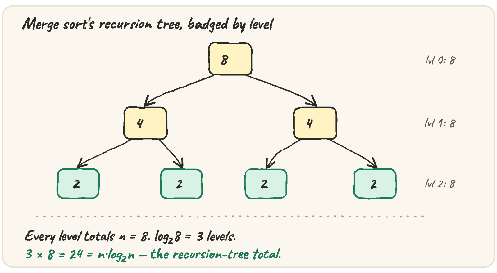
Every non-leaf level adds up to 8: one merge of 8, two of 4, four of 2. The leaves write nothing. So the total is n per level times log₂ n levels, 8 × 3 = 24 here. That is the recursion-tree method: draw the tree, total each level, add the levels. Now check it by counting instead of drawing:

python

They match exactly for powers of two. The recursion tree was not an estimate; it was an exact count.

Three shapes of tree

Change what each call does and the tree keeps its shape, but the badges change. Keep two calls on halves and make the combine step cost n² instead of n:

T(n) = 2\,T(n/2) + n^2

Labels are sizes; badges are each call's own work, first with an n combine, then n².

watch it move · tree

Same tree, different badges. With an n combine every level ties; with an n² combine each level is half the one above, so the root dominates.

With f(n) = n the root merges 8 items and each half merges 4. Binary tree, 15 nodes, height 4. At node 8.

1 / 6

Now go back to split3: three calls on halves with a linear combine, $T(n) = 3\,T(n/2) + n$ . A node with three children needs a graph:

watch it move · graph

Calls triple while sizes only halve, so each level costs more than the one above and the leaves decide.

The root does 4 work and hands out three halves. 13 nodes, 12 edges, directed. At 4. 4: w=4.

1 / 3

Shrinking levels, tied levels, growing levels: those are the only three shapes.

The master theorem is the three shapes in one line

For $T(n) = a\,T(n/b) + n^k$ , level i has $a^i$ calls, each on a problem of size $n/b^i$ , each doing $(n/b^i)^k$ work. So level i costs

a^i \cdot \left(\frac{n}{b^i}\right)^k = n^k \cdot \left(\frac{a}{b^k}\right)^i

Everything depends on the ratio $a / b^k$ between one level and the next:

compare	levels	cost	example
$a < b^k$	shrink	$\Theta(n^k)$	$2T(n/2) + n^2$ is $\Theta(n^2)$
$a = b^k$	tie	$\Theta(n^k \log n)$	merge sort: $2 = 2^1$ , so $\Theta(n \log n)$
$a > b^k$	grow	$\Theta(n^{\log_b a})$	$4T(n/2) + n$ is $\Theta(n^2)$

In the last row the leaves decide: branching a, depth $\log_b n$ , so $a^{\log_b n} = n^{\log_b a}$ leaves. Binary search is a tie with $k = 0$ , so $\Theta(\log n)$ .

The combine costs n² and each call gets half the input. How many calls a can a function make before the leaves start to decide its cost? Compare the leaf count $n^{\log_2 a}$ with the combine's n²:

calls `a`	leaves grow like	who decides
2	$n^{1}$	the combine: $\Theta(n^2)$
3	$n^{1.58}$	the combine: $\Theta(n^2)$
4	$n^{2}$	a tie: $\Theta(n^2 \log n)$
5	$n^{2.32}$	the leaves: $\Theta(n^{2.32})$
8	$n^{3}$	the leaves: $\Theta(n^3)$

At a = 4 the two meet, because log₂ 4 = 2 = k: the tie case. With fewer calls the combine wins; with more, the leaves win.

Summing the levels by hand

The same level-by-level sum as a loop, for merge sort on 8 items. Watch calls double while size halves:

step through it

1n, calls, size, total = 8, 1, 8, 0

2while size >= 1:

3 level = calls * size

4 total += level

5 calls *= 2

6 size //= 2

7print(total)

It counts the 8 leaves too, so it prints 32, which is $n \log_2 n + n$ . What a leaf costs changes lower-order terms, never the shape.

When the master theorem does not fit

The theorem needs equal pieces that shrink by a factor. When your code does not have that shape, the recursion tree still works.

Uneven splits. A pivot that always lands 10% of the way in gives calls of n/10 and 9n/10. Every level still totals at most n, and there are $\log_{10/9} n$ levels: still $O(n \log n)$ , with a bigger constant.

Shrinking by subtraction. Quick sort on a sorted list with a last-element pivot makes one call on n − 1 items. The tree is a single path, n levels deep, and the levels cost n, n − 1, n − 2, …:

What does this print?

def T(n):
    if n <= 1:
        return 1
    return T(n - 1) + n

print(T(10))

Two calls that shrink by one, T(n) = 2T(n − 1) + 1, give $2^n$ leaves: naive Fibonacci and subset search.

❓ Cross-question — "Is the base case irrelevant?" For the Big-O, yes: it only sets a constant on each leaf. For real speed it matters, which is why production sorts switch to insertion sort below about 16 to 64 items.

Idioms & real-world patterns

Write the recurrence in a comment

A loop inside a recursive function runs once per call. When you review recursive code, write # T(n) = 2T(n/2) + n above it: one line tells the next reader the cost.

Slicing is part of f(n)

items[:mid] copies half the list, which is linear work added to f(n). In merge sort that changes nothing. In binary search it turns $T(n) = T(n/2) + 1$ into $T(n) = T(n/2) + n$ , which is $\Theta(n)$ : no faster than a scan. Pass lo and hi instead.

⚡ Advanced — the substitution method

A recursion tree gives a guess; induction proves it. Assume $T(n/2) \le c\,\tfrac{n}{2} \log_2 \tfrac{n}{2}$ and substitute: $T(n) \le c\,n\log_2 n - c\,n + n \le c\,n \log_2 n$ for $c \ge 1$ .

Quick practice

What does this print?

a, b, k, n = 3, 3, 2, 9
levels, calls, size = [], 1, n
while True:
    levels.append(calls * size ** k)
    if size == 1:
        break
    calls *= a
    size //= b
print(levels)

broken — fix it

Splitting into thirds with three recursive calls should give T(27) = 108. This prints 40, because the code only ever makes one call instead of three.

🎯 Your turn

Write level_work(n, a, b, k), the cost lab's first instrument. For $T(n) = a\,T(n/b) + n^k$ , return the total work on each level of the recursion tree, root first, including the level of size-1 calls. n is a power of b.

level_work(8, 2, 2, 1) → [8, 8, 8, 8], merge sort: every level ties
level_work(8, 2, 2, 2) → [64, 32, 16, 8], the root dominates
level_work(8, 4, 2, 1) → [8, 16, 32, 64], the leaves dominate

Hint — it is the trace loop above, with a, b and k in place of 2, 2 and 1.

Then press ▶ Run, tap the Live App try chips, and hit ✓ Check.

Recurrences & the Recursion Tree

Recurrences & the Recursion Tree

From code to a recurrence

Drawing the recursion tree

Three shapes of tree

The master theorem is the three shapes in one line

Summing the levels by hand

When the master theorem does not fit

Idioms & real-world patterns

Write the recurrence in a comment

Slicing is part of f(n)

⚡ Advanced — the substitution method

Quick practice

🎯 Your turn

Practice — level up