
Capstone — the Tunebox Cost Lab
In short: instrument a function with a counter on its dominant operation,
measure it at sizes that double, and the growth rate falls out of the
ratio between neighbouring counts (×2 linear, ×4 quadratic). For a precise
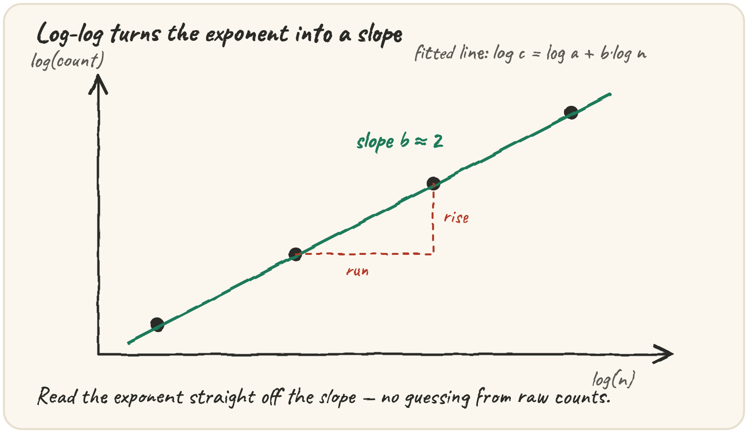
exponent, take logs of both n and the count: on a log-log plot a power law
a·n^b becomes a straight line whose slope is b. The lab then checks that
slope against the bound you proved on paper — and settles the n log n vs
n^1.1 ambiguity by dividing the counts by each candidate model and seeing
which one leaves a flat line.
You now have two ways of knowing what code costs. On paper: read a recurrence off the code, solve it with a recursion tree, account for spikes with a bank of tokens, average over random pivots. In the machine: count the operations while the code runs. Each one checks the other. A proof with a slip in it disagrees with the count, and a count taken on an unlucky input disagrees with the proof.
The capstone puts them together in one instrument. The cost lab takes a function from sections 1 to 6, runs it on inputs of growing size, counts its real operations, fits a curve to the counts, and reports the exponent. You then compare that exponent with the bound you derived.
Step 1: instrument
Timing with a stopwatch measures your laptop. Counting measures the code. Pick the operation that dominates, the one inside the innermost loop, and add a counter there. For insertion sort from section 3 that is the shift:
A reversed list of four needs 6 shifts, a sorted one needs none. Which input you measure on matters as much as how you count, so the lab always states it: worst case (reversed), best case (sorted), or a seeded random input for the average.
Step 2: sweep n by doubling
Measure at n, 2n, 4n, 8n. Doubling makes the growth rate readable straight off the ratio between neighbouring counts: about 2 means linear, 4 means quadratic, 8 means cubic, and slightly more than 2 means n log n.
counts = [120, 496, 2016, 8128]
ratios = [round(counts[k + 1] / counts[k], 1) for k in range(len(counts) - 1)]
print(ratios)Here is the lab's sweep running on your insertion sort, filling in its results
table as it goes. Each row is one size; the last column is the doubling ratio.
Swap in a different function: replace the body of measure with your merge
sort's write count or a BFS on a bigger grid, and watch the ratio column change.
Your sweep, one row per size. A ratio settling at 4 says quadratic before any curve is fitted.
Step 3: fit a power law
Ratios are easy to read, but noisy data needs a single number. If the cost is , taking logarithms turns it into a straight line:
So plot against and the slope is the exponent. With two measurements, the slope is just rise over run. Step through it:
With many measurements, fit the best straight line by least squares, the same method as in regression:
A slope is only meaningful on the log scale. Fit the raw numbers and you get the wrong kind of answer:
The counts are exactly n², so the fitted exponent should print 2.0. It prints 92.61, the slope of the raw counts: "about 93 more steps per extra item", which is not an exponent at all.
Step 4: the verdict, and why n log n looks like n^1.1
Run the lab on four of your functions, each on inputs chosen to match the bound you proved:
Insertion sort comes out near 2, the append and BFS near 1. Merge sort comes out around 1.18, which is not a sign that it is . Over a range of sizes, looks like a power law whose exponent is a little above 1, and the extra part shrinks slowly as the range moves to larger n. An exponent alone cannot tell from . The lab settles it the other way round: fit each candidate model and keep the one that leaves the smallest error.
import math

ns = [1024, 2048, 4096]
counts = [n * int(math.log2(n)) for n in ns]
print([round(c / n, 1) for c, n in zip(counts, ns)])The same division, done on merge sort's real counts:
Divide the counts by each candidate model. The right model leaves a constant; the wrong one leaves a trend.
Merge sort's measured writes at five sizes, each double the last. 3 by 5 table. At row 0, column 0 — value 384. 5 of 15 cells filled.
That is the boss exercise: compare the models n, n log n and n² directly
against the counts, rather than trusting one exponent.
❓ Cross-question — "Why not just time it?" Timings mix in the interpreter, the cache, the garbage collector and whatever else the machine is doing, and they differ between runs. They are the right tool for "is it fast enough?" Counts are the right tool for "does it grow the way I proved?" The lab uses counts so that the same code gives the same answer every time.
Idioms & real-world patterns
Measure the worst case on purpose
Random inputs show the average. Bugs in production come from the worst case: the sorted chart, the listener with a million followers. Include the input your proof says is worst, and check that the count matches.
Stop a sweep before it hurts
Doubling grows fast. Put a budget on the total operations counted and stop the sweep when the next size would exceed it. A quadratic function at n = 10⁶ takes a lot longer than you want to wait.
⚡ Advanced — residuals
After fitting, compute each measurement's relative error against the fitted curve. If the errors drift steadily in one direction with n, the model has the wrong shape, however good the exponent looks. That drift is the signal that separates from a power law.
Quick practice
counts = [100, 800, 6400, 51200]
ratios = [round(counts[k + 1] / counts[k], 1) for k in range(len(counts) - 1)]
print(ratios)The counts triple... no, they go ×8 each time n doubles, so the ratios should read [8.0, 8.0, 8.0]. This prints [0.12, 0.12, 0.12] — correct in spirit (constant, so still a clean power law) but inverted, which would be misread as "shrinking" work.
🎯 Your turn
Write fit_exponent(ns, counts), the lab's curve fitter. Given sizes and the
operation counts measured at them (all positive), return the least-squares slope of
log(count) against log(n), rounded to 2 decimal places.
fit_exponent([10, 20, 40, 80], [100, 400, 1600, 6400])→2.0fit_exponent([100, 200, 400], [300, 600, 1200])→1.0
Then use the exercises to build the rest of the lab: doubling ratios, instrumented specimens, a model chooser, and the report that says which Tunebox feature breaks first.
Press ▶ Run, tap the Live App try chips, and hit ✓ Check.